Written on September 13, 2019 8 min read

(Insights) Of Rabbits and Foxes

A quick overview of the Lotka-Volterra model.

Brief motivation

Among the different domains of Maths I’ve come across so far, one that made a lasting impression on me is the dynamic of populations, with the prey-predator model of Lotka-Volterra.

Why is so ? Because this model, somehow quite simple, allow us to play with some interesting and beautiful mathematical concepts while being applied to a funny situation. Simplicity, elegance, enjoyment; what more a mathematician could ask for ?

The Lotka-Volterra model

The goal of the Lotka-Volterra model is to represent the evolution through time of two populations: the preys (rabbits) and the predators (foxes). To do so, it introduce a very simple system of equations that can be either deterministic or stochastic, but in both cases it is working the same way.

In our model, only three things can happen: preys reproduce; predators reproduce by eating preys; predators die. We will thus have only three parameters in this model, corresponding to each action. Let’s note $x$ the preys and $y$ the predators. The prey reproduction parameter is $\alpha$, the predator reproduction is $\beta$ and the predator death paramater is $\gamma$.

Deterministic approach

We consider we have a constant prey reproduction rate, so the corresponding evolution of preys is given by $\alpha x(t)$. Likewise, the predator death rate is constant so the corresponding evolution term is $\gamma y(t)$. As the reproduction of predator is linked to the number of preys, the corresponding term is $\beta x(t) y(t)$ and depends both on the density of preys and predators. In the end, the system describing the evolution of preys and preddators is quite simple and given by:

\[\left\{ \begin{array}{r c l} x'(t) &=& \alpha x(t) - \beta \, x(t) \, y(t) \\ y'(t) &=& \beta x(t) y(t) - \gamma y(t) \end{array} \right.\]

There are few explicit solutions to this system: if at some point in time, there are no preys anymore so $x(t)$ = 0, then the number of predators quickly decreases to 0. It’s quite logical because they cannot eat anymore, but you can also see that because the equation then is $y’(t) = - \gamma y(t)$ so $y(t) = y(0) \text{e}^{-\gamma t}$. If this time there are no more predators i.e. $y(t) = 0$, then the preys strive: $x(t) = x(0) \text{e}^{\alpha t}$. A more interesting situation is when, at $t = t_0, x(t_0) = \gamma / \beta$ and $y(t_0) = \alpha / \beta$, then the system stays stable so that the number of preys and predators remains constant.

But now, let’s simulate all that! Hopefully, libraries solving ordinary differential equations do exist, so we do not need to code everything. In R, which I will use here, the deSolve library does a pretty good job. We just have to create the function containing our ODEs, choose the parameter values and the initial number of preys and preddators and we are done.

library(deSolve)
library(ggplot2)

LV <- function(Time, State, Pars) {
  with(as.list(c(State, Pars)), {
    dPrey        <- alpha * Prey - beta * Prey * Predator
    dPredator    <- beta * Prey * Predator - gamma * Predator
    return(list(c(dPrey, dPredator)))
  })
}

pars  <- c(alpha  = 0.15, beta = 0.04, gamma  = 0.3)

ini  <- c(Prey = 10, Predator = 10)
times <- seq(0, 200, by = 1)
out   <- ode(ini, times, LV, pars)

data = as.data.frame(out)
ggplot(data = data, aes(x=time)) + geom_line(aes(y=Predator, colour= "Foxes"), linetype="longdash", lwd=0.5) +
  geom_line(aes(y=Prey, colour = "Rabbits"), lwd=0.5) + ggtitle("Lotka-Volterra model") +
  scale_colour_manual("Legend", breaks = c("Foxes", "Rabbits"), values = c("#F8766D", "#00BFC4")) + ylab("Population") + xlab("Time") +
  theme(legend.position = c(0.93, 0.93)) + ylim(0,18)

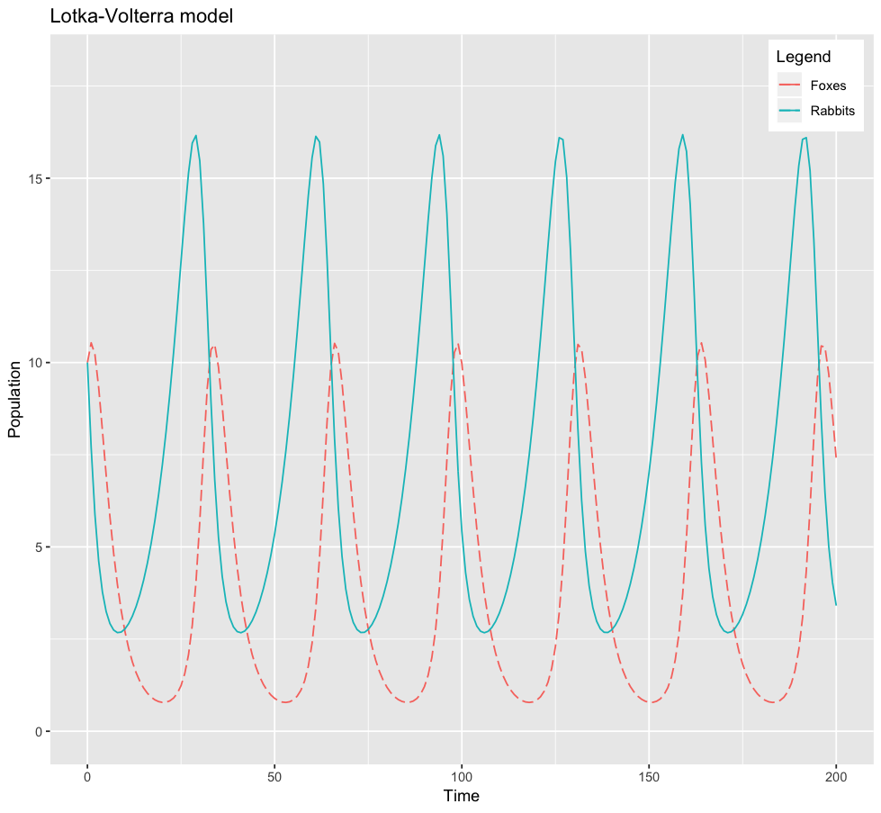
With the parameters we’ve chosen ($\alpha = 0.15, \beta = 0.04, \gamma = 0.3$), we obtain the following evolution:

Stochastic approach

The stochastic approach is funnier (well at least for me). In this set up, the three possible actions we had (prey reproduction, predator death or predator eating prey) are converted into probable actions. We thus have:

\[\left\{ \begin{array}{l c l} \mathbb{P}(X(t+dt) = x+1; Y(t+dt)=y | X(t)=x; Y(t)=y) &=& \alpha x \, \text{d}t = q_1 \, \text{d}t \\ \mathbb{P}(X(t+dt) = x-1; Y(t+dt)=y+1 | X(t)=x; Y(t)=y) &=& \beta x y \, \text{d}t = q_2 \, \text{d}t \\ \mathbb{P}(X(t+dt) = x; Y(t+dt)=y-1 | X(t)=x; Y(t)=y) &=& \gamma y \, \text{d}t = q_3 \, \text{d}t \end{array} \right.\]

Now that we have our model described, we would like to simulate it. The Gillespie algorithm is designed to deal with problems like ours, so that’s what we will use. Before we do so, in the next paragraph, I’ll try to illustrate why and how this algorithm works.

$(X(t), Y(t))$ is a continuous Markov chain with a countable state space I. We can have a closer look to the transition rate matrix of this chain, an object which will help us describe when a the system will change from one state to another. This matrix $Q = (q_{i,j \in I})$ satisfies:

• $\forall \; i \neq j, q_{i,j}$ is the speed at which the system changes from state $i$ to state $j$
• $\forall \; i \in I, q_{i,i} = - \sum_{j \neq i} q_{i,j}$

In our case, from a fixed state $(x, y)$, we can only access three different states: $(x+1, y)$, $(x-1, y+1)$ or $(x, y-1)$ with repectively $q_1, q_2$ and $q_3$ as transition rate. What is nice with this matrix is that a well-known property of continuous time Markov chains states that the holding time in state $i$ until the next jump, noted $S_{i}$ follows an exponential law of parameter $-q_{i,i} = q_1 + q_2 + q_3$.

Thanks to that, we thus know when the next jump / change of state will occur, given the state $i$ we are in. We just have to know which event will take place: prey reproduction, predator reproduction or predator death. This is quite easy: event $j$ will occur with probability $\frac{q_{i,j}}{q_1 + q_2 + q_3}$. So for example, the prey reproduction event occur with probability $\frac{q_1}{q_1 + q_2 + q_3}$.

And we are done! This was all the point of the Gillespie algorithm, that we can sum up like this:

• 1) Initialise your problem: $t=0, \, x(0) = x, \, y(0) = y$
• 2) Compute your transition rates: $q_1 = \alpha x, \, q_2 = \beta x y, \, q_3 = \gamma y$ and $q = q_1 + q_2 + q_3$
• 3) Simulate whan the next event will occur: $s \sim \mathcal{E}(q)$ and $t \leftarrow t + s$
• 4) Simulate which event will occur: $\mathbb{P}(\text{event } i) = q_i / q$
• 5) Change your number of preys and predators accordingly: if $i = 1, x \leftarrow x + 1 ;$ if $i = 2, x \leftarrow x-1$ and $y \leftarrow y+1 ; $ and if $i = 3, y \leftarrow y-1$
• 6) Repeat from step 2)

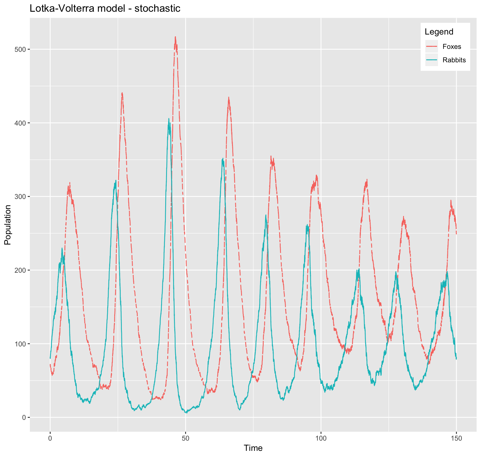
We can do it the good old way: coding entirely this small algorithm. You can find it just below, along with the plot of what we obtain for one simulation.

library(reshape2)
library(ggplot2)

# Initialization
param <- c(0.5, 0.003, 0.3)
x0 <- 80
y0 <- 70
t_max <- 150

# Function to simulate the problem
simu_x_y <- function(param,x,y,t_max){
  t <- 0
  Prey <- c(x)
  Predator <- c(y)
  Time <- c(0)
  i <- 2
  
    while(t <= t_max){
      q1 <- param[1]*x
      q2 <- param[2]*x*y
      q3 <- param[3]*y
      q <- q1 + q2 + q3
        
      s <- rexp(1, rate = q)*(q >0)
      if (q==0){break}

      q_sort = sort(c(q1,q2,q3))
      q_order <- order(c(q1,q2,q3))
      u <- runif(1, min=0, max=1)
      if (u<q_sort[1]/q){r <- as.name(paste0("q", q_order[1]))}
      if (u>=q_sort[1]/q & u<(q_sort[1] + q_sort[2])/q){r <- as.name(paste0("q", q_order[2]))}
      if (u >= (q_sort[1] + q_sort[2])/q) {r <- as.name(paste0("q", q_order[3]))}
    
      if (r == "q1" & x > 0){x <- x + 1}
      else if(r=="q1" & x == 0){x = 0}
      if (r == "q2" & x > 0 & y > 0){
      x <- x - 1
      y <- y + 1
      }else if( (r=="q2" & x == 0) | (r=="q2" & y == 0) ){x = 0
      y = 0}
      if (r == "q3" & y > 0){y <- y - 1}else if(r=="q3" & y == 0){y = 0}
    
      Prey[i] <- x
      Predator[i] <- y
      Time[i] <- t
      i <- i+1
      t <- t + s
    }
    return(data.frame(Time, Prey, Predator))
  }

out <- simu_x_y(param, x0, y0, t_max)
ggplot(out, aes(x = Time)) + geom_line(aes(y=Predator, colour="Foxes"), linetype="longdash", lwd=0.5) +
  geom_line(aes(y=Prey, colour="Rabbits"), lwd=0.5) + ggtitle("Lotka-Volterra model - stochastic") +
  scale_colour_manual("Legend", breaks = c("Foxes", "Rabbits"), values = c("#F8766D", "#00BFC4")) + ylab("Population") +
  theme(legend.position = c(0.93,0.93))

The stochastic approach of this Lotka-Volterra model just scratches the surface of the all the maths behind the continous time Markov chains, which are pretty nice. The advantage of that is you can understand the prey and predators dynamic without digging too much into maths theory, and with a rather short algorithm, simulate the model. But as the theory about Markov chains really worth it, I hope this brief overview of the subject piqued your curiosity, like it did for me.